Linear Algebra

• The element-wise product of two matrices is known as the Hadamard product.
• A system of linear equations is $Ax = b$.
• If we know the inverse of the matrix $A$, we can solve for $x$. Note that in practice, we usually do not use $A^{-1}$ to solve for $b$. This is because the inverse of a matrix can be represented with only limited precision on a digital computer. Algorithms that make use of the value of $b$ can usually obtain a more accurate estimate of $x$.
• In order for $A^{-1}$ to exist, the system of linear equations must have exactly one solution for every value of $b$. Determining whether $Ax = b$ has a solution amounts to testing whether bis in the span of the columns of $A$.
• In order for the system $Ax = b$. to have a solution for all values of $b$, the column space of $A$ must be the entire set of vectors $R^{m}$. Note that this means that the matrix $A$ must have at least $m$ linearly independent columns.
• In order for the matrix to have an inverse, $Ax = b$ must have at most one solution for each value of $b$. To that end, we need to ensure that the matrix $A$ has at most $m$ columns. Otherwise, there is more than one way of parameterizing each solution. Together with the previous conditions, this means that $A$ must be square.
• Another way of thinking about this is, when a matrix is invertible, the map it represents is invertible. This means that it is an isomorphism between linear spaces, and we know this is possible if and only if the linear spaces' dimensions are the same. Which implies that $m = n$, and the matrix is square.
• A square matrix with linearly dependent columns (i.e. no inverse) is known as singular.
• Basically, a matrix is invertible if the linear mapping that it represents is both surjective (onto: every element in the co-domain is mapped to by at least one element in the domain) and injective (one-to-one).
• Why does a matrix need to be square in order to be invertible?
• In machine learning, we measure the size of vectors using a function called the norm. Any function $f$ that satisfies three properties is a norm:
  • If $f(x) = 0$, then $x$ is the zero vector.
  • $f(x + y) \leq f(x) + f(y)$, also known as the triangle inequality.
  • For all scalars $\alpha$, $f(\alpha x) = |\alpha|f(x)$.
• The $L^{2}$ norm, or Euclidean norm is often denoted $||x||$.
• What is the gradient of the squared $L^{2}$ norm?
• The squared $L^{2}$ norm may be undesirable because it increases very slowly near the origin. In cases where we need to discriminate between elements that are exactly zero and elements that are small but nonzero, we often use the $L^{1}$ norm, which grows at the same rate in all locations.
• We can measure the size of a matrix using the Frobenius norm, which is the square root of the sum of each element of the matrix squared.
• Diagonal matrices only have nonzero elements along the diagonal. They are interesting because:
  • Multiplying a vector $x$ by a diagonal matrix is very efficient (we simply scale the elements of the $x$).
  • Inverting a square diagonal matrix is also very efficient. The inverse exists only if each diagonal entry is nonzero.
• A symmetric matrix is any matrix that is equal to its own transpose. They often arise when the entries are generated by some function of two arguments that does not depend on the order of the arguments. For example, a matrix of distance measurements where $A_{i, j}$ gives the distance from point i to point j. Clearly, $A_{i, j} = A_{j, i}$.
• An orthogonal matrix is a square matrix whose rows are mutually orthonormal and whose columns are mutually orthonormal. In other words, $A^{T}A = AA^{T} = I$. Critically, this means that the inverse of the matrix is equal to its transpose.
• Eigendecomposition involves breaking a matrix into a set of eigenvectors and eigenvalues. An eigenvector of a square matrix $A$ is a nonzero vector $v$ such that multiplication by $A$ alters only the scale of $v$. In other words, $Av = \lambda v$. Since any eigenvector multiplied by a scalar is also an eigenvector, we usually only look for unit eigenvectors. We can concatenate all of the eigenvectors to form a matrix $V$ with one eigenvector per column. Likewise, we can concatenate the eigenvalues to form a vector $\lambda$. So, we can now write: $AV = Vdiag(\lambda)$. By multiplying each side of the equation by $V^{-1}$ on the right, we obtain the eigendecomposition: $A =Vdiag(\lambda)V^{-1}$. An example of computing the eigendecomposition of a matrix can be found here.
• Constructing matrices with specific eigenvalues and eigenvectors allows us to stretch space in desired directions.
• Every real symmetric matrix is guaranteed to have an eigendecomposition, but it might not be unique. By convention, an eigendecomposition is unique only if all of the eigenvalues are unique.
• A matrix is singular if and only if any of the eigenvalues are zero (explained here, which also explains why diagonal matrices are interesting).
• Eigenvectors and eigenvalues explained visually.
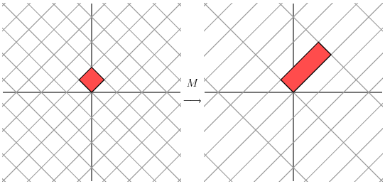
• Note that rotation matrices have no eigenvectors or eigenvalues, since they simply rotate space. There are no transformed points that are along their original line through the origin. Also, note that the eigenvectors of a symmetric matrix corresponding to different eigenvalues are always orthogonal. Put another way, it turns out that we may always rotate the Cartesian plane in the domain such that a symmetric matrix acts by stretching (and perhaps reflecting) in two orthogonal directions. This is pictured below:

• The sign of the eigenvalues of a matrix can be used to classify it into one of four categories: a matrix is said to be positive semidefinite when it can be obtained as the product of a matrix by its transpose. This implies that a positive semidefinite matrix is always symmetric. This family of matrices includes correlation, covariance, and cross-product matrices. Positive semidefinite matrices are interesting because $x^{T}Ax$ is guaranteed to be greater than or equal to zero. Intuitively, this means that the mapped vector does not "go in the other direction" from the original.
  • Positive definite: all eigenvalues are positive
  • Positive semidefinite: all eigenvalues are positive or zero
  • Negative definite: all eigenvalues are negative
  • Negative semidefinite: all eigenvalues are negative or zero
• The singular value decomposition (SVD) provides another way to factorize a matrix into singular vectors and singular values. Every real matrix has a SVD, even non-square matrices. It is written as the product of three matrices: $A = UDV^{T}$.
• If $A$ is $m\times n$, then $U$ is $m\times m$, $D$ is $m\times n$, and $V$ is $n\times n$. $U$ and $V$ are both orthogonal. $D$ is diagonal and not necessarily square. The elements of $D$ are known as the singular values of the matrix $A$. The SVD can be used to generalize matrix inversion to non-square matrices.
• Understanding singular value decomposition.
• The SVD can be used for things like data compression and noise reduction. In a way, the SVD discovers redundancy in a matrix and provides a format for eliminating it. The number of non-zero singular values equals the rank of the matrix. Remember that the rank of a matrix denotes the number of linearly independent columns.
• The Moore-Penrose Pseudoinverse gives us a way to solve a system of linear equations $Ax = b$ when $A$ is non-square (and therefore, not directly invertible).
• The trace operator gives the sum of all of the diagonal entries of a matrix.
• The determinant of a square matrix is a function mapping matrices to real scalars. It is equal to the product of all of the eigenvalues of the matrix (the area of the parallelogram spanned by the eigenvectors of the matrix). The absolute value of the determinant can be thought of as a measure of how much multiplication by the matrix expands or contracts space.