Machine Learning Basics

• Machine learning tasks are usually described in terms of how the machine learning system should process an example. An example is a collection of features that have been qualitatively measured from some object or event that we want the machine learning system to process. We typically represent an example as a vector $x$ where each entry is another feature.
• Usually we are interested in how well the machine learning algorithm performs on data that it has not seen before, since this determines how well it will work when deployed in the real world. We therefore evaluate our performance measures using a test set of data that is separate from the data used for training the machine learning system.
• Roughly speaking, unsupervised learning involves observing several examples of a random vector $x$ and attempting to implicitly or explicitly learn $p(x)$. Supervised learning involves observing several examples of a random vector $x$ and an associated value or vector $y$ and learning $p(y\mid x)$. However, many machine learning technologies can be used to perform both tasks. Due to the chain rule of probability, we can solve the unsupervised problem by splitting it into $n$_ _supervised learning problems. Alternatively, we can solve the supervised learning problem by using traditional unsupervised learning technologies to learn the joint distribution $p(x, y)$. An example of the first transformation is neural autoregressive distribution estimation (NADE), which is explained in the following blog post. An example of the second transformation is a naive Bayes classifier, which is explained in the following Wikipedia article.
• Some machine learning algorithms do not just experience a fixed dataset. For example, reinforcement learning algorithms interact with an environment, so there is a feedback loop between the learning system and its experiences.
• One common way of describing a dataset is with a design matrix, which contains a different training example in each row. Each column corresponds to a different feature.
• Parameters are values that control the behavior of the system. We often think of parameters as a set of weights that determine how each feature affects the prediction. If a feature receives a positive weight, then increasing the value of that feature increases the value of our prediction and vice-versa. If a feature's weight is large in magnitude, then it has a large effect on the prediction. If a feature's weight is zero, it has no effect on the prediction.
• Often times, the parameters of a model include a bias term, which pushes the output of the model's transformation towards the value of the bias in the absence of any input.
• One of the simplest machine learning problems is linear regression, which can be solved directly with the normal equations. The derivation of these equations can be found in the following blog post.
• The ability of a machine learning system to perform well on previously unseen data is called generalization. What separates machine learning from optimization is that we would like both the training error and test error to be low.
• The train and test data are generated by a probability distribution over datasets called the data generating process. We typically make a set of assumptions known collectively as the i.i.d. assumptions that state that the examples in each dataset are independent from each other and that the train set and test set are identically distributed (drawn from the same probability distribution). We call this shared underlying distribution $p_{data}$.
  • An example of a dataset that is not i.i.d. would be, if we measured some variables on a bunch of children but chose kids who were in particular classes in particular schools: kids in the same class are likely to be more similar to each other than kids in different classes. This is explained in further detail in the following article.
  • Why is the i.i.d. assumption important in machine learning?
• During training, we want to:
  • Make the training error small, otherwise we will experience underfitting.
  • Make the gap between the training and test error small, otherwise we will experience overfitting.
• Parametric models (such as linear regression) learn a function described by a parameter vector whose size is finite and fixed before any data is observed. Non-parametric models (such as nearest neighbor regression) have no such limitation.
• The ideal model will still incur some error on many problems. The error incurred by the model making predictions from the true distribution $p(x, y)$ is called Bayes error. The Bayes error of a classifier is the probability of misclassification.
• The no free lunch theorem implies that we must design machine learning algorithms to perform well on specific tasks.
• We can regularize a model by adding a penalty called a regularizer to the cost function. Regularization allows the model to express a preference for one function over another. It is a more general way of controlling a model's capacity than including or excluding members from the hypothesis space.

Regularization is any modification we make to a learning algorithm that is intended to reduce its generalization error but not its training error.

• If learned on the training set, hyperparameters would always choose the maximum possible model capacity, resulting in overfitting. For example, we can always fit the training set better with a higher-degree polynomial and a weight decay setting of 0 than we could with a lower-degree polynomial and a positive weight decay setting. To solve this problem, we use a validation set of examples that the training algorithm does not observe.
• $k$-fold cross-validation lets you use all of the examples in the estimation of the mean test error, which can be useful when the dataset is small.
• Point estimation is the attempt to provide the single "best" prediction of some quantity of interest, which can be a single parameter or a vector of parameters in some parametric model (i.e. weights). A point estimator or statistic is any function of the data.
  • As an example of a point estimate, assume you wanted to estimate the mean time it takes 12-year-olds to run 100 yards. The mean running time of a random sample of 12-year-olds would be an estimate of the mean running time for all 12-year-olds. Thus, the sample mean, $M$, would be a point estimate of the population mean, $\mu$.
• The bias of an estimator is defined as the expected value of the estimated value of $\theta$ minus the true underlying value of $\theta$ used to define the data-generating distribution. An estimator with 0 bias is said to be unbiased. An estimator is said to be asymptotically unbiased if the bias goes to 0 in the limit that the number of data points goes to infinity.
• Derivation of estimators of the variance of a Gaussian distribution.
• Unbiased estimators are usually desirable, but they are not always the "best" estimators. Sometimes we use biased estimators that possess other important properties.
• Another property of an estimator that we might want to consider is how much we expect it to vary as a function of the data sample. The square root of the variance of an estimator is called the standard error. The standard error provides a measure of how we would expect the estimate we compute from data to vary as we independently resample the dataset from the underlying data generating process. The standard error of the mean is very useful in machine learning experiments. We often estimate the generalization error by computing the sample mean of the error on the test set.
• A statistic describes a sample whereas a parameter describes an entire population. The SE uses statistics whereas the standard deviation uses parameters.
• What is the standard error of the mean?
• Often times, the variance of an estimator decreases as a function of $m$, the number of examples in the dataset.

• The mean squared error (MSE) measures the overall expected deviation - in a squared error sense - between the estimator and the true value of the parameter $\theta$. Evaluating the MSE incorporates both the bias and the variance. Desirable estimators are those with small MSE that manage to keep both their bias and variance somewhat in check. The MSE can be written as the sum of the variance of the estimator and the squared bias of the estimator. A proof of this property can be found in the following Wikipedia article.
  

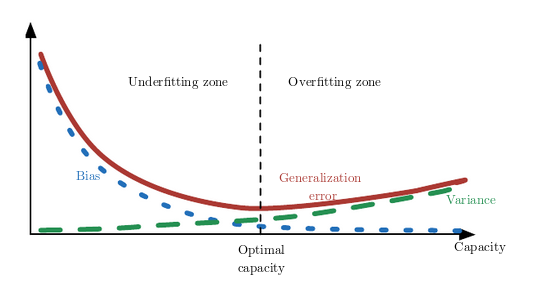
• We usually wish that as the number of data points $m$ in our dataset increases, our point estimates converge to the true value of the corresponding parameters. This condition in known as consistency. Consistency ensures that the bias induced by the estimator diminishes as the number of data examples grow. However, the reverse is not true - asymptotic unbiasedness does not imply consistency.

• Where do these estimators come from? We would like to have some principle from which we can derive specific functions that are good estimators for different models. The most common such principle is the maximum likelihood principle.

• Maximum likelihood estimation (MLE) is a method for determining the parameters of a model. The parameter values are found such that they maximize the likelihood that the process described by the model produced the data that was actually observed. To use MLE, we should have a good idea about which model to use, which usually comes from having some domain expertise. For example, we might say that a particular dataset can be adequately described by a Gaussian distribution. In this case, we simply need to find the model parameters ($\mu$ and $\sigma^{2}$) that best fit our data. We want to calculate the total probability of observing all of the data: the joint probability distribution of all observed data points. This can be very difficult, so we make the assumption that each data point is generated independently of the others. This means that the total probability is the product of observing each data point individually: the product of the marginal probabilities. We can usually take this expression and differentiate with respect to the parameters in order to find a global maximum. Note that this product over many probabilities can be prone to numerical underflow. To obtain a more convenient but equivalent optimization problem, we observe that taking the logarithm of the likelihood does not change its $\arg\max$ but does transform a product into a sum. All of this is detailed in the following article.

• One way to interpret MLE is to view it as minimizing the dissimilarity between the empirical distribution defined by the training set and the model distribution. The degree of dissimilarity between the two distributions is measured by the KL divergence.
• We can therefore view MLE as an attempt to make the model distribution match the empirical distribution defined by the training data.
• MLE can readily be generalized to estimate a conditional probability $P(y\mid x; \theta)$. This forms the basis for most supervised learning. Note that according to several Discord users, the notation here isn't quite accurate. In particular, $y$ isn't really conditioned on $x$. Rather, the notation is saying: "consider the distribution of $y$ as if you are given all of the $x$'s already."
• There are two approaches to learning model parameters:
  • Frequentist statistics: we estimate a single value of $\theta$ and make all predictions thereafter based on that one estimate (everything above falls into this category).
  • Bayesian statistics: we consider all possible values of $\theta$ when making a prediction. In the Bayesian perspective, the dataset is directly observed and so is not random. On the other hand, the true parameter $\theta$ is unknown and thus is represented as a random variable. A very detailed explanation of Bayesian statistics and an example of prior / posterior distributions can be found in the following article.

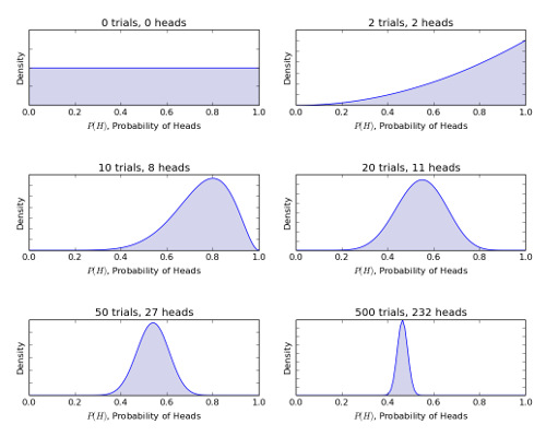
• As an aside, in Bayesian statistics we often talk about prior and posterior probabilities:
  • Bayes' theorem connects these two modalities. An excellent example of this can be found in the following Quora post ("winds" noun vs. verb). An example of starting with a prior and updating it based on new evidence can be found in the following blog post, which uses a baseball batting average analogy. Basically, we might start with a beta distribution centered around a "typical" batting average for a professional player (say, 0.27). Then, as we obtain more evidence about a particular player, we can shift and skew this distribution to reflect the new information.
  • The posterior is your belief once additional information is collected. It tells you how you'd revise those beliefs in the presence of data.
  • The prior is what you believe about some quantity at a particular point in time. It tells you the relative likelihood of different values of some quantity in the absence of data. Typically, the machine learning practitioner selects a prior distribution that is quite broad (i.e. with high entropy) to reflect a high degree of uncertainty in the value of parameter before observing any data.
• The maximum a posteriori (MAP) point estimate chooses the point of maximal posterior probability.
• A simple example of MAP.
• MLE and MAP are similar in that they compute a single estimate of some parameter instead of a full distribution. The only thing that differs (in terms of optimization) is the inclusion of the prior in MAP. Otherwise, they are identical. What that means is, the likelihood is weighted with some value coming from the prior. It can be shown that MAP with a Gaussian prior on a model's weights is proportional to the familiar weight decay penalty. MAP Bayesian inference with a Gaussian prior on the weights thus corresponds to weight decay.
• MLE vs. MAP explained.
• An example of both a frequentist and Bayesian view of linear regression can be found in the following article, which also explains why MAP Bayesian inference with a Gaussian prior on the weights corresponds to the familiar weight decay formulation.
• What is the connection between MLE and cross-entropy loss in deep learning?
• Most supervised learning algorithms are based on estimating a probability distribution $p(y\mid x)$. We can do this simply by using MLE to find the best parameter vector $\theta$ for a parametric family of distributions $p(y\mid x;\theta)$. If we are performing binary classification, the mean of the distribution must always be between 0 and 1. One way to account for this is to use the logistic sigmoid function to squash the output of the linear function into the interval $(0, 1)$ and interpret that value as a probability. In this scenario, there is no closed-from solution for finding the optimal setting of the weight matrix. Instead, we must search for it by maximizing the log-likelihood (or equivalently, minimizing the negative log-likelihood) using gradient descent.
• The support vector machine (SVM) is similar to logistic regression in that it is driven by a linear function. Unlike logistic regression, the SVM does not provide probabilities. The SVM predicts that the positive class is present when the output of the linear function is positive and vice-versa.

Of all possible decision boundaries that could be chosen to separate the dataset for classficiation, the SVM chooses the decision boundary that is most distant from the points closest to the decision boundary from both classes.

• One key innovation associated with SVMs is the kernel trick:
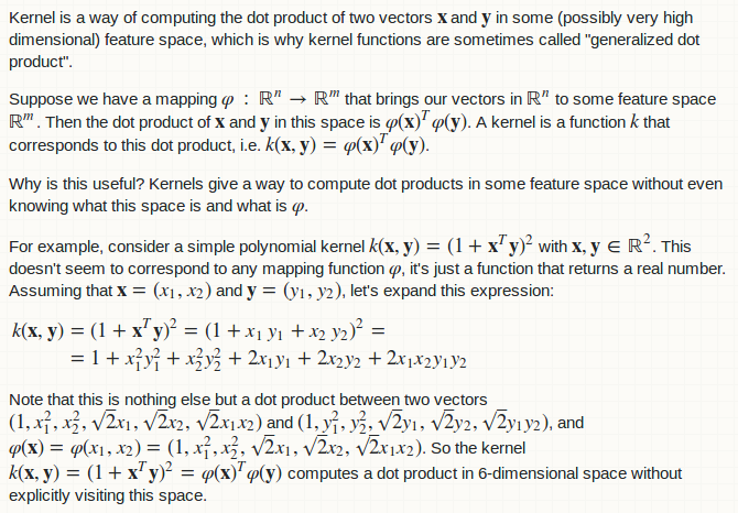
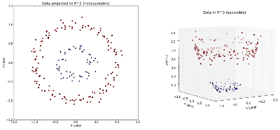
  • The main idea is, if a dataset isn't linearly separable in an $n$-dimensional space, it might be linearly separable in a higher dimensional space.
  • The kernel trick essentially defines the transformed space in terms of the original space without ever defining what the transformation function actually is. A kernel is a way of computing the dot product between two vectors in some (possibly very high-dimensional) feature space. Kernel functions are sometimes called a "generalized dot product." An example of how a kernel function computes such a dot product without ever explicitly visiting the higher-dimensional space can be found in the following post.
  • The kernel-based function is exactly equivalent to pre-processing the data by applying a non-linear function to the input $x$ and then learning a linear model in the new transformed space. The most common kernel is the radial basis function (RBF).
  • The mathematics behind the SVM are explained in detail in the following blog post.

• Another type of learning algorithm that breaks the input space into regions and has separate parameters for each region is the decision tree. Space is subdivided into non-overlapping regions with a one-to-one correspondence between leaf nodes and input regions. Each leaf node usually maps every point in its input region to the same output.
• A classic unsupervised learning task is to find the "best" representation of the data - generally, one that preserves as much information about the input as possible while obeying some penalty or constrained aimed at keeping the representation simpler than the input itself. Three of the most common ways of defining a simpler representation are:
  • Lower-dimensional representations
  • Sparse representations
  • Independent representations
• Principal components analysis (PCA) learns an orthogonal, linear transformation of the data that projects an input $x$ to a representation $z$. PCA finds a representation (through a linear transformation) where $Var(z)$ is diagonal - in other words, the individual elements of $z$ are mutually uncorrelated. It attempts to disentangle the unknown factors of variation underlying the data. This disentangling takes the form of finding a rotation of the input space that aligns the principal axes of variance with the basis of the new representation space associated with $z$.
  • The principle components of a design matrix $X$ are given by the eigenvectors of $X^{T}X$.
  • The principle components may also be obtained via singular value decomposition (they are the right singular vectors of $X$).
  • The principal components (eigenvectors) correspond to the direction (in the original $n$-dimensional space) with the greatest variance in the data.
  • PCA is a way of identifying patterns in data and expressing the data in such a way as to highlight its similarities and differences.
• $k$-means clustering transforms an input $x$ into a $k$-dimensional one-hot code vector $h$, where $h_{i} = 1$ when $x$_ _belongs to cluster $i$. This vector $h$ is an example of a sparse representation because the majority of its entries are zero for every input. The clustering problem is inherently ill posed in the sense that there is no single criterion that measures how well a clustering of the data corresponds to the real world. Also, there may be many equally valid clusterings that all correspond well to some property of the real world. For example, we might have a dataset that consists of red cars, red trucks, gray cars, and gray trucks. One clustering could be: {red cars, red trucks} and {gray cars, gray trucks}. Another might be: {red cars, gray cars} and {red trucks, gray trucks}. These issues illustrate some of the reasons that we may prefer a distributed representation to a one-hot representation. A distributed representation could have two attributes for each vehicle (color and car vs. truck).
• The cost function used by a machine learning algorithm often decomposes as a sum over the training examples of some per-example loss function. The insight of stochastic gradient descent is that the gradient on the cost function with respect to the parameter $\theta$ is an expectation that can be approximated by using a small set of samples called a minibatch.
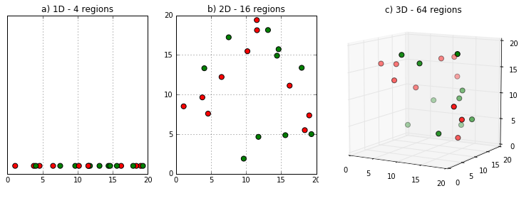
• Many machine learning problems become exceedingly difficult when the number of dimensions in the data is high. This phenomenon is known as the curse of dimensionality. Basically, if we hold the size of our dataset constant and gradually increase the dimension of the space in which we plot our data, the sampling of the space becomes more and more sparse. This makes it very difficult for the model to generalize to unseen examples. This is explained in detail in the following article.
• We informally discuss prior beliefs as being expressed implicitly by choosing algorithms that are biased towards choosing some class of functions over another. Among the most widely used of these implicit "priors" is the smoothness prior or local constancy prior, which states that the function we learn should not change very much within a small region. In other words, if we know a good answer for an input $x$, then that answer should probably be good in the neighborhood of $x$. The smoothness assumption and the associated non-parametric learning algorithms work extremely well as long as there are enough examples for the learning algorithm to observe high points on most peaks and low points on most valleys of the true underlying function to be learned.
• A local kernel can be thought of as a similarity function that performs template matching by measuring how closely a test example resembles each training example.
• The core idea in deep learning is that we assume that the data was generated by the composition of features, potentially at multiple levels in a hierarchy.
• In machine learning, a manifold is a connected region. Mathematically, it is a set of points associated with a neighborhood around each point. From any given point, the manifold locally appears to be a Euclidean space. For example, we experience the surface of the world as a 2D plane, but it is in fact a spherical manifold in 3D space.
• What is manifold learning?
• PCA finds the directions along which the data has maximum variance in addition to the relative importance of these directions. For example, suppose that we feed a set of 3D points that all lie on a 2D plane to PCA. PCA will return two vectors that span the plane along with a third vector that is orthogonal to the plane. The first two vectors will be given a positive weight, while the third will be given a weight of zero. Manifold learning algorithms can be viewed as a non-linear version of PCA. PCA projects the data onto some low-dimensional surface, but this is restrictive in the sense that all of those surfaces are linear. What if the best representation lies on some weirdly shaped surface? PCA will totally miss this.

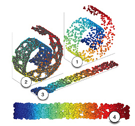
• The assumption that the data lies along a low-dimensional manifold may not always be correct or useful. In the context of AI tasks involving images, sound, or text, the manifold assumption is at least approximately correct.
• The first observation in favor of the manifold hypothesis is that the probability distribution over images, text strings, and sounds that occur in real life is highly concentrated:
  • For example, if we generate a document by picking letters uniformly at random, the probability of getting a meaningful English-language text is almost zero. This is because most of the long sequences of letters do not correspond to a natural language sequence: the distribution of natural language sequences occupies a very little volume in the total space of sequences of letters.
  • The manifold hypothesis is important because it (partially) explains why we are able to learn anything at all using deep learning. If this hypothesis holds true, then the task of classification is fundamentally to separate a bunch of tangled manifolds.
  • Part of this is due to the fact that the layers of a neural network are a homeomorphism. In other words, each layer stretches and squishes space to form a new representation, but it never cuts, breaks, or folds it. Intuitively, we can say that each layer preserves topological properties (a set will be connected afterwards if it was before, etc.). This is explained in detail in the following article.
• When the data lies on a low-dimensional manifold, it can be most natural for machine learning algorithms to represent the data in terms of coordinates on the manifold rather than in terms of coordinates in the original $n$-dimensional space. In everyday life, we can think of roads as 1D manifolds embedded in 3D space. We give directions to specific addresses in terms of address numbers along these 1D roads, not in terms of coordinates in 3D space.