Deep Feedforward Networks

• It is best to think of feedforward networks as function approximation machines that are designed to achieve statistical generalization.
• Linear models (such as logistic regression and linear regression) have the obvious defect that the model capacity is limited to linear functions, so the model cannot understand the interaction between any two input variables. To extend linear models to represent non-linear functions of $x$, we can apply the linear model not to $x$ itself but to a transformed input $\phi(x)$, where $\phi$ is a non-linear transform. We can think of $\phi$ as providing a new representation for $x$.
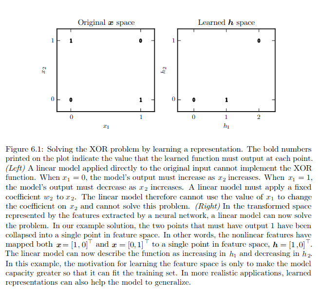
• The excerpt below explains why a simple linear model cannot solve the XOR problem, which serves as the motivation for non-linear activation functions in deep feedforward networks:

• In modern neural networks, the default recommendation is to use the rectified linear unit, or ReLU, defined by the activation function $g(z) = \max (0, z)$.
  • How is the ReLU activation function able to approximate non-linear functions?
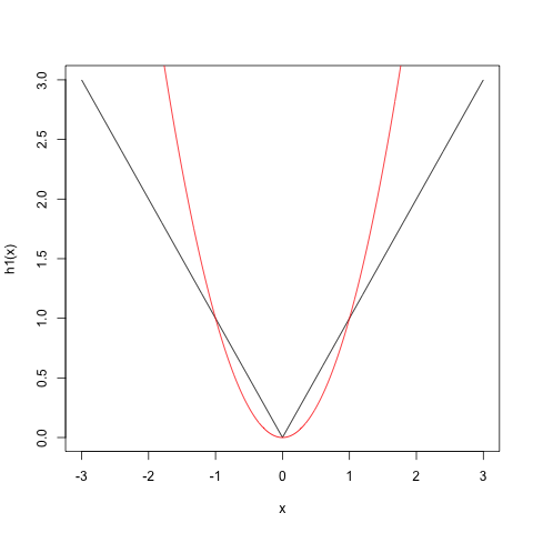
  • Suppose we want to approximate the function $f(x) = x^{2}$ using ReLUs $g(ax + b)$. One approximation might look like $h_{1}(x) = g(x) + g(-x) = |x|$. This is shown in the first graph below.
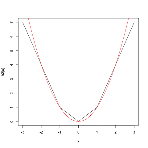
  • This obviously isn't a very good approximation. We can add more terms to improve the approximation, like: $h_{2}(x) = g(x) + g(-x) + g(2x - 2) + g(-2x + 2)$. This is shown in the second graph below.

• The largest difference between the linear models we have seen so far and neural networks is that the non-linearity of a neural network causes most interesting loss functions to become non-convex. This means that neural networks are usually trained by driving the cost function to a very low value rather than an absolute global minimum.
• Most modern neural networks are trained using maximum likelihood. This means that the cost function is simply the negative log-likelihood, equivalently described as the cross-entropy between the training data and the model distribution.
• We can think of learning as choosing a function rather than merely choosing a set of parameters.
  • As a review, note that:
    • Probability lets us predict unknown outcomes based on known parameters.
    • Likelihood lets us predict unknown parameters based on known outcomes.
    • This is explained in the following article.
    • An example of using MLE to solve linear regression can be found in the following article.
    • Consider the problem of binary classification. Maximizing the (log) likelihood of the data under a Bernoulli distribution is equivalent to minimizing the binary cross-entropy. This can be extended to the multi-class case using softmax cross-entropy and the so-called multinoulli likelihood. This is derived in the following Quora post.
    • The difference between MLE and cross-entropy is that MLE represents a structured, principled approach to modeling and training, whereas cross-entropy simply represents a special case of this applied to a type of classification problems that people typically care about.
    • The connection between MLE and expectation is explained in the following post.
    • During MLE, we almost always convert the joint probability distribution of our dataset into a sum, using logarithms. We do this because a sum is a lot easier to optimize, since the derivatives of a sum is the sum of its derivatives:
      • By using a sum, we can load each training example (one at a time), compute its partial derivatives, and accumulate those gradients.
      • If we were using a product, all of the training examples are "entangled," so we would need to load the entire training set to calculate the product. Only then would we be able to compute the partial derivatives of all of the parameters and apply an optimization step.
    • This is why we use the logarithm: to get rid of the product signs.
    • Of course, maximizing the log-likelihood of the parameters given a dataset is strictly equivalent to minimizing the negative log-likelihood. All of the bullet points above are discussed in the following article.
    • The following article contains a table of different regularization strategies and their probabilistic interpretations as a prior used during MAP estimation.
• Any kind of neural network unit that may be used as an output can also be used as a hidden unit. Throughout this book, we suppose that the feedforward network provides a set of hidden features defined by $h = f(x;\theta)$. The role of the output layer is then to provide some additional transformation from the features to complete the task that the network must perform.
• There are many different types of output layers:
  • Linear unit: this unit is based on an affine transformation $W^{T}h + b$. It is often used to produce the mean of a conditional Gaussian distribution. Maximizing the log-likelihood is then equivalent to minimizing the mean squared error.
  • Sigmoid unit: this unit is often used for binary classification. In this case, the maximum likelihood approach is to define a Bernoulli distribution over $y$ conditioned on $x$. Because the cost function used with maximum likelihood is $-\log P(y\mid x)$, the $\log$ in the cost function undoes the $\exp$ of the sigmoid. This helps prevent the saturation that would normally occur with a different loss function, such as mean squared error.
  • Softmax unit: this unit is often used to represent a probability distribution over a discrete variable with $n$ possible values. This can be seen as an extension of the sigmoid unit, where we used exponentiation and normalization to give us a Bernoulli distribution controlled by the sigmoid function.
    • Overall, unregularized maximum likelihood will drive a model to learn parameters that drive the softmax to predict the fraction of counts of each outcome observed in the training set. In practice, limited model capacity and imperfect optimization will mean that the model is only able to approximate these fractions.
    • If we have $n$ classes, a linear layer before the softmax unit will actually overparametrize the distribution. The constraint that the $n$ outputs must sum to 1 means that only $n - 1$ parameters are necessary: the probability of the $n$-th value may be obtained by subtracting the first $n - 1$ probabilities from 1. To account for this, we can impose a requirement that one element of $z$ be fixed at 0.
    • This is exactly what the sigmoid unit does: defining $P(y = 1\mid x) = \sigma(z)$ is equivalent to defining $P(y = 1\mid x) = softmax(z)_{1}$ with a 2-dimensional $z$ and $z_{1} = 0$. Note that in practice, there is rarely much different between using the overparametrized version or the restricted version.
  • Other output units: in general, we can think of the neural network as representing a function whose outputs are not direct predictions. Instead, this function $f(x;\theta) = \omega$ provides the parameters for a distribution.
    • For example, we may wish to learn the variance of a conditional Gaussian for $y$ given $x$.
    • We often want to perform multimodal regression, that is, to predict real values from a conditional distribution $p(y\mid x)$ that can have several different peaks in $y$ space for the same value of $x$. In this case, a Gaussian mixture is a natural representation for the output. Neural networks with Gaussian mixtures as their output are often called mixture density networks (MDN).
      • A typical neural network can only predict one output value for each input. A MDN can predict a range of different values for each input.
      • To do this, the network predicts an entire probability distribution for the output. Practically speaking, this means that the last layer of the network will have 3 outputs for each of the $k$ Gaussians: $p(c = k\mid x)$ for the $k$-th Gaussian (these will be forced to sum to 1), the mean $\mu_{k}$, and the standard deviation $\sigma_{k}$.
      • All of this is explained in the following blog post, which also contains a TensorFlow implementation of a MDN.
      • Gradient-based optimization of conditional Gaussian mixtures can be unreliable, in part due to the divisions (by the variance) which can be numerically unstable. This occurs when the variance gets to be very small for a particular example, yielding very large gradients. One solution is to clip gradients.
      • Gaussian mixture outputs are effective in generative models of speech and movement of physical objects. The MDN strategy gives the network a way to represent multiple output modes and to control the variance of its output, which is crucial for obtaining a high degree of quality in these real-valued domains.
• Some types of hidden units, such as those including ReLUs, are not actually differentiable at all input points. In practice, this is not an issue because neural network training algorithms do not usually arrive at a local minimum of the cost function but instead, merely reduce its value significantly. Because we do not expect training to actually reach a point where the gradient is 0, it is acceptable for the minima of the cost function to correspond to points with an undefined gradient.
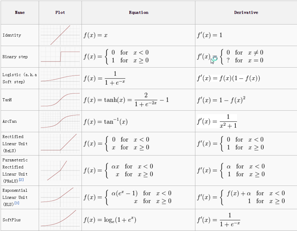
• There are many different types of hidden units:
  • Rectified linear unit: this unit is typically used on top of an affine transformation $h = g(W^{T}x + b)$. When initializing the parameters of the transformation, it is good practice to set all elements of $b$ to a small positive value, such as 0.1. Doing so makes it very likely that the ReLU will be initially active for most inputs in the training set. One drawback to ReLUs is that they cannot learn via gradient-based methods on examples for which their activation is zero. The leaky ReLU or parametric ReLU variations attempt to fix this.
  • Maxout unit: this unit generalizes the ReLU by dividing $z$ into groups of $k$ values. Each maxout unit then outputs the maximum element of one of these groups. This provides a way of learning a piecewise linear function that responds to multiple directions in the input $x$ space.
    • When $k = 2$, a maxout neuron computes the function $\max(w_{1}^{T}x + b_{1}, w_{2}^{T} + b_{2})$.
    • Both ReLU and leaky ReLU are a special case of this form. For example, a ReLU sets $w_{1} = b_{1} = 0$.
    • A maxout neuron enjoys all of the benefits of a ReLU unit and does not have its drawbacks (dead ReLUs). However, using maxout neurons doubles the number of parameters needed for every single neuron.
  • Sigmoid and hyperbolic tangent units: these units compute $\sigma(z)$ and $\tanh(z)$, respectively. Their use as hidden units in feedforward networks is discouraged because they can lead to poor training dynamics. Sigmoidal activation functions are more common in recurrent networks, probabilistic models, and autoencoders, which have additional requirements that rule out the use of piecewise linear activation functions.
  • Other hidden units: softmax units are usually used as an output unit but may sometimes be used as a hidden unit. They can be interpretted as a kind of "switch." A few other common hidden unit types include:
    • Radial basis function
    • Softplus
    • Hard tanh

• The word architecture refers to the overall structure of the network: how many units it should have and how these units should be connected to each other.
• The universal approximation theorem states that a feedforward network with a linear output layer and at least one hidden layer with any activation function can approximate any continous function on a closed and bounded subset of $R^{n}$ with any desired nonzero amount of error, provided that the network is given enough hidden units. A proof of this theorem can be found in the following blog post.
• Even though this theorem means that a network can (in theory) represent any function that we are trying to learn, this doesn't mean that it will in practice. Learning can fail for two reasons:
  • The optimization algorithm used for training may not be able to find the value of the parameters that corresponds to the desired function.
  • The training algorithm might choose the wrong function as a result of overfitting.
• In many circumstances, using a deeper model can reduce the number of units required to represent the desired function and reduce the amount of generalization error.

Choosing a deep model encodes a very general belief that the function we want to learn should involve the composition of several simpler functions. This can be interpreted from a representation learning point of view as saying that we believe that the learning problem consists of discovering a set of underlying factors of variation that can, in turn, be described in terms of other, simpler underlying factors of variation.

• The term back-propagation is often misunderstood as meaning the _whole _learning algorithm for multi-layer neural networks. Actually, back-propagation refers only to the method for computing the gradient, while another algorithm (like SGD) is used to perform learning using this gradient.
• To facillitate back-propagation, we use the notion of a computational graph, where each node represents either:
  • A variable (scalar, vector, matrix, tensor, or otherwise).
  • An operation (function of one or more variables).
• Each node has a set of consumers (children) and inputs (parents).
• Back-propagation is a highly efficient algorithm that computes the chain rule of calculus with a specific order of operations. The chain rule states that for a real number $x$ and two functions $y = g(x)$ and $z = f(g(x)) = f(y)$, the derivative of $z$ with respect to $x$ is: $\frac{dz}{dx} = \frac{dz}{dy}\frac{dy}{dx}$. The chain rule is explained in detail in the following Khan Academy article.
• We can generalize the chain rule beyond the scalar case. Suppose that $x\in R^{m}$ and $y\in R^{n}$. Let $g$ be an intermediate function that maps from $R^{m}$ to $R^{n}$. Finally, let $f$ be a function that maps from $R^{n}$ to $R$. The gradient of $z$ with respect to $x$ can be written as the product of a Jacobian matrix $\frac{dy}{dx}$ and a gradient $\bigtriangledown_{y}z$. The back-propagation algorithm consists of performing such a Jacobian-gradient product for each operation in the graph:
  • Usually we apply the back-propagation algorithm to tensors of arbitrary dimensionality, not just vectors. Conceptually, this is the exact same. The only difference is how the numbers are arranged in a grid to form a tensor. We could imagine flattening each tensor into a vector before we run back-propagation, computing a vector-valued gradient, and then reshaping the gradient back into a tensor. In this view, back-propagation is still just multiplying Jacobians by gradients.
  • One of the hardest parts about understanding back-propagation in neural networks is knowing how to take derivatives with respect to functions that accept or return matrices. The following PDF from Erik Learned-Miller explains how to approach this.
• Computation graphs are explained in detail in the following blog post and on the course website for Stanford's CS231n. In particular, there are two ways of calculating derivatives on computational graphs:
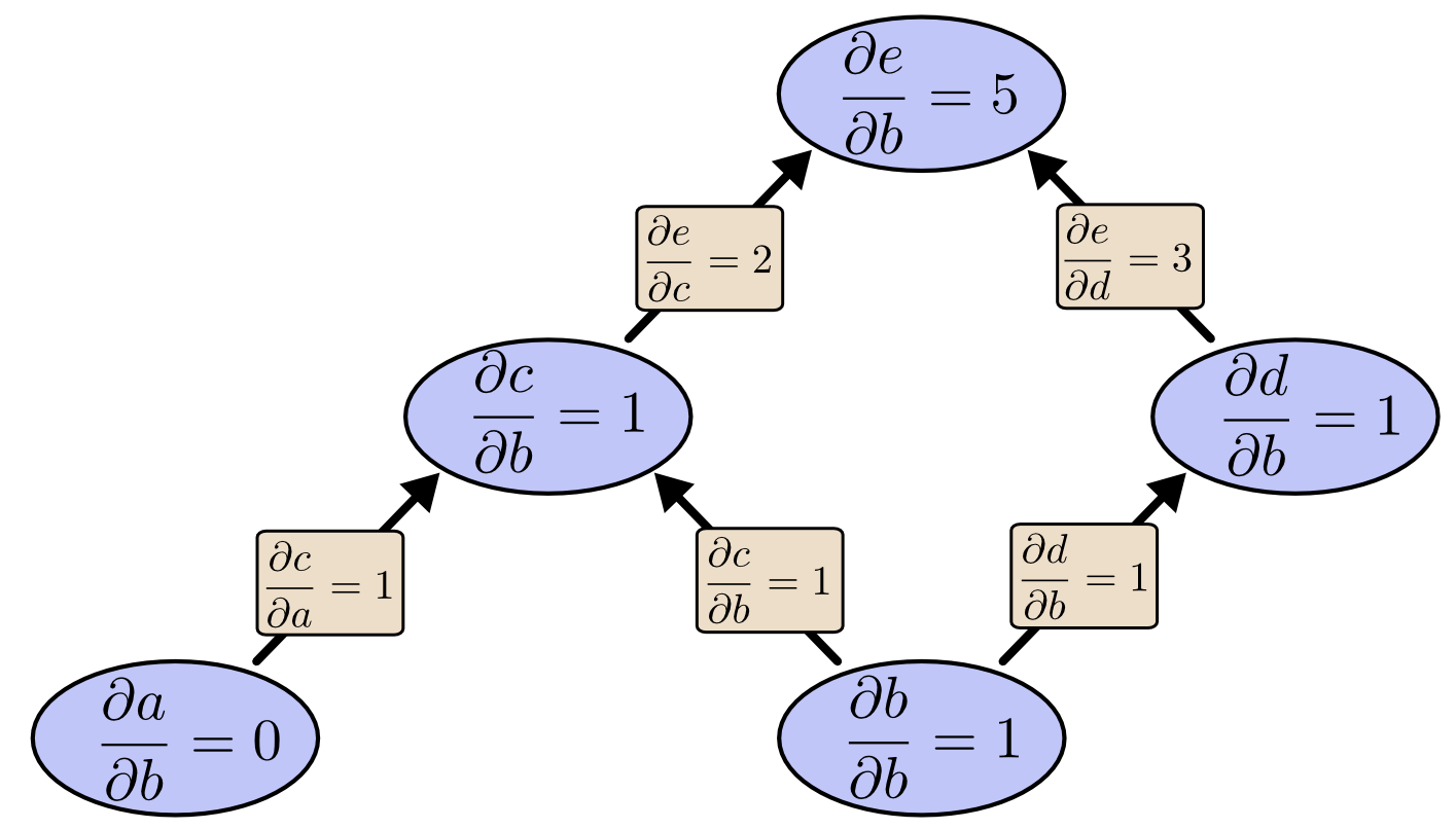
  • Forward-mode differentiation tracks how one input affects every node by applying the operator $\frac{\partial}{\partial{X}}$ to every node for some input $X$.
  • Reverse-mode differentiation tracks how every node affects one output by applying the operator $\frac{\partial{Z}}{\partial}$ to every node. The advantage of reverse-mode differentiation is that it gives us the derivative of some output $Z$ with respect to every node. This means that we can calculate all of the partial derivatives necessary for back-propagation in one pass. This is what PyTorch uses internally in its autograd module. A worked out example of reverse-mode differentiation can be found in the following post.
• Both modes involve "factoring" the edges of the graph, so as to avoid the combinatorial explosion in the number of possible paths. An example of forward-mode differentiation (from node $b$ upwards) can be seen in the image below.

• Computational graphs operate on symbols, or variables that do not have specific values. These algebraic and graph-based representations are called symbolic representations. When we actually use or train a neural network, we must assign specific values to these symbols. We replace a symbolic input to the network $x$ with a specific numeric value, such as $[1, 2, 3]^{T}$. Some approaches to back-propagation take a computational graph and a set of numerical values for the inputs to the graph, then return a set of numerical values describing the gradient at those input values. We call this approach symbol-to-number differentiation.
• Another approach is to take a computational graph and add addtional nodes to the graph that provide a symbolic description of the desired derivatives. This is the approach taken by Theano and TensorFlow and is known as symbol-to-symbol differentiation. The advantage here is that the derivatives are described in the same language as the original expression. Any subset of the graph can be evaluated using specific numerical values at a later time.
• So, to compute the gradient of some scalar $z$ with respect to one of its ancestors $x$ in the graph, we begin by observing that the gradient with respect to $z$ is given by $\frac{dz}{dz} = 1$. We can then compute the gradient with respect to each parent of $z$ in the graph by multiplying the current gradient by the Jacobian of the operation that produced $z$. We continue multiplying by Jacobians, traveling backward through the graph in this way until we reach $x$.

For any node that may be reached by going backward from $z$ through two or more paths, we simply sum the gradients arriving from different paths at that node.

• The computational graph API:
  • get_operation: returns the operation that computes $V$
  • get_consumers: returns the list of variables that are children of $V$ in the graph
  • get_inputs: returns the list of variables that are parents of $V$ in the graph
• Each operation is also associated with a bprop operation that computes a Jacobian-vector product, as discussed earlier. This method should always pretend that all inputs are distinct, even if they are not. For example, if the mul operator is passed two copies of $x$ to compute $x^{2}$, the bprop method should still return $x$ as the derivative with respect to both inputs. The back-propagation algorithm will later add both of these arguments together to obtain $2x$, which is the correct total derivative on $x$.
• The field of automatic differentiation is concerned with how to compute derivatives algorithmically. Back-propagation is only one approach to automatic differentiation. It is a special case of a broader class of techniques called reverse mode accumulation.
• The cost of training can be reduced by simplifying the computational graph constructed by back-propagation. Implementations such as Theano and TensorFlow use heuristics based on matching known simplification patterns to iteratively simplify the graph.
• When the number of outputs of the graph is larger than the number of inputs, it is sometimes preferable to use another form of automatic differentiation called forward mode accumulation. This approach avoids the need to store the values and gradients for the whole graph.
• Reverse-mode and forward-mode differentiation are covered in Colah's blog post above as well as in the following article, which contains a basic implementation of forward mode accumulation in Python and Rust. Another example of reverse-mode differentiation can be found in the following blog post. The biggest takeaway is:

In forward-mode automatic differentiation, we have to run through the entire graph for each parameter whose gradient we wish to compute. In effect, the cost of this method scales linearly as O(n) where n is the number of input variables.

In reverse-mode automatic differentiation, we have to run through the entire graph for each output variable whose gradient we wish to compute. In effect, the cost of this method scales linearly as O(m) where m is the number of output variables.

• In the deep learning community, computational graphs are usually represented by explicit data structures created by specialized libraries. This approach has the drawback of requiring the library developer to define the bprop method for every operation and thus, limiting the user to only those operations that have been defined. However, this approach has the benefit of allowing customized back-propagation rules to be developed for each operation, enabling the developer to improve speed and/or stability.
• In typical deep learning applications, it is infeasible to compute (or even represent) the entire Hessian matrix of second derivatives. Instead, a more common approach is to use Krylov methods, which are a set of iterative techniques for performing various operations such as approximately inverting a matrix.