Optimization for Training Deep Models

• The goal of a machine learning algorithm is to reduce the expected generalization error or risk. Here, the expectation is taken over the true underlying distribution $p_{data}$. If we knew the true distribution $p_{data}(x, y)$, risk minimization would be an optimization task solvable by an optimization algorithm. When we do not know $p_{data}(x, y)$ but only have a training set of samples, we have a machine learning problem.
• The simplest way to convert a machine learning problem back into an optimization problem is to minimize the expected loss on the training set. This empirical risk can be written as $\frac{1}{m}\sum_{i=1}^{m}L(f(x^{(i)};\theta), y^{(i)})$. This process is known as empirical risk minimization. However, it has several problems.
  • Empirical risk minimization is prone to overfitting.
  • In many cases, empirical risk minimization is not feasible, since many useful loss functions have no useful derivatives or the derivative is either zero or undefined everywhere. This makes it difficult (or impossible) to optimize with gradient descent.
  • The two problems above mean that we rarely use empirical risk minimization. Instead, we use a slightly different approach in which the quantity that we actually optimize is even more different from the quantity that we truly want to optimize. For example, instead of using a 0-1 loss, we might use the negative log-likelihood of the correct class.
  • This is known as a surrogate loss function.
• The connection between maximum likelihood estimation and neural networks is explained here.
• Optimization algorithms that use the entire training set are called batch gradient methods. Optimization algorithms that use only a single example at a time are called stochastic methods. Most algorithms fall somewhere in between. These are called minibatch methods.
  • Larger batch sizes provide a more accurate estimate of the gradient but with less than linear returns. This follows from the fact that the standard error of the mean estimated from $n$ samples is given by $\frac{\sigma}{\sqrt{n}}$, where $\sigma$ is the true standard deviation of the value of the samples. The denominator shows that there are less than linear returns to using more examples to estimate the gradient. For example, we can compare two hypothetical estimates of the gradient: one based on 100 examples and another based on 10,000 examples. The latter requires 100 times more computation than the former but reduces the standard error of the mean only by a factor of 10.
  • The standard error of the mean is explained in detail in the following article.
  • It is crucial that the minibatches be selected randomly. Ideally, two subsequent minibatches of examples should be independent of each other. It is often necessarily to shuffle the training set before selecting minibatches.
  • Minibatch stochastic gradient descent follows the gradient of the true generalization error as long as no examples are repeated. Most implementations shuffle the dataset once and then pass through it multiple times. On the first pass, each minibatch is used to compute an unbiased estimate of the true generalization error. On the second pass, the estimate becomes biased because it is formed by resampling values that have already been used.
  • The reason why the expected value of the gradient of a minibatch in SGD is equal to the true empirical gradient is explained in the following Quora post.
• There are several large challenges in neural network optimization.
  • Often times, the Hessian matrix is ill-conditioned, which is explained in the following Quora post. Essentially, a poorly conditioned Hessian matrix causes problems for first-order optimization methods like SGD, which will need to follow a very zigzag path to the minimum.
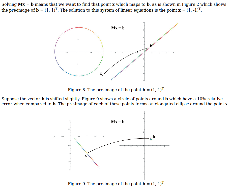
    • Ill conditioned and well conditioned matrices are discussed in the following article. Basically, an ill conditioned system $Mx = b$ may be very sensitive to small changes in either the matrix $M$ or the vector $b$. This means that a relatively small change in either can result in a significant change in the solution $x$. This is shown in the image below.
  • With non-convex functions such as neural networks, it is possible to have many local minima due to weight space symmetry. This is known as the model identifiability problem. Another example is, in any rectified linear or maxout network, we can obtain an equivalent model by scaling all of the incoming weights and biases of a unit by $\alpha$ if we also scale all of its outgoing weights by $\frac{1}{\alpha}$.
    • However, all of these local minima are equivalent to each other in cost function value. As a result, these local minima are not a problematic form of non-convexity.
    • Local minima can be problematic if they have high cost in comparison to the global minimum.
  • For many high-dimensional non-convex functions, local minima (and maxima) are rare compared to saddle points, where the Hessian matrix has both positive and negative eigenvalues. For many classes of random functions, saddle points are extremely common in higher-dimensional spaces.
    • To understand the intuition behind this behavior, observe that the Hessian matrix at a local minima only has positive eigenvalues. Imagine that the sign of each eigenvalue is generated by flipping a coin. In a single dimension, it is easy to obtain a local minimum by tossing a coin and getting heads once. In an $n$-dimensional space, it is exponentially unlikely that all $n$ coin tosses will be heads.
    • The gradient can often become very small near a saddle point, but empirically, SGD seems to be able to escape these flat regions in many cases.
    • However, for Newton's method, which is designed to solve for a point where the gradient is zero, saddle points clearly constitute a problem. This explains why second-order methods have no succeeded in replacing gradient descent for neural network training.
  • Neural networks with many layers often have extremely steep regions resembling cliffs, which result from the multiplication of several large weights together. Fortunately, this can be avoided by using gradient clipping. Recurrent neural networks often suffer from this problem.
  • Repeated application of the same parameters can also give rise to difficulties. For example, suppose that a computational graph contains a path that consists of repeatedly multiplying by a matrix $W$. If $W$ has an eigendecomposition, it is straightforward to see that $W^{t} = V diag(\lambda)^{t}V^{-1}$. Any eigenvalues $\lambda_{i}$ that are not near an absolute value of 1 will either explode if they are greater than 1 or vanish if they are less than 1. Gradients through such a graph are also scaled according to $diag(\lambda)^{t}$. This is known as the vanishing / exploding gradient problem.
    • This procedure is very similar to the power method algorithm, which is used to find the largest eigenvalue of a matrix via repeated multiplication.

• In practice, it is necessary to gradually decrease the learning rate over time. This is because the SGD gradient estimator introduces a source of noise (the random sampling of minbatches) that does not vanish even when we arrive at a minimum. Usually, we decay the learning rate linearly until iteration $\tau$ as follows: $\epsilon_{k} = (1 - \alpha)\epsilon_{0} + \alpha\epsilon_{\tau}$, where $\alpha = \frac{k}{\tau}$.

The learning rate may be chosen by trial and error, but it is usually best to choose it by monitoring learning curves that plot the objective function as a function of time.

• To study the convergence rate of an optimization algorithm, it is common to measure the excess error $J(\theta) - \min_{\theta}J(\theta)$, which is the amount by which the current cost function exceeds the minimum possible cost. When SGD is applied to a convex problem, the excess error is $O(\frac{1}{\sqrt{k}})$ after $k$ iterations. Related to excess error are the concepts of Cramer-Rao Bound and Fischer Information, which are explained in the following post.
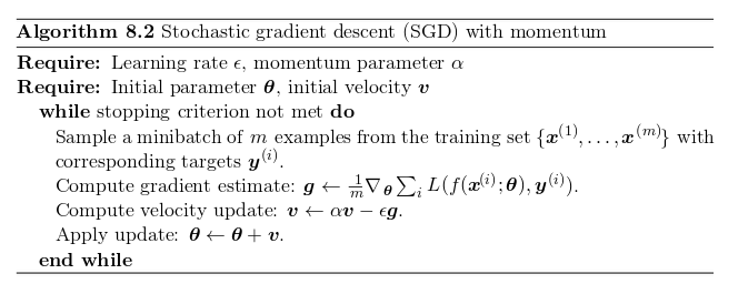
• The momentum algorithm accumulates an exponentially decaying moving average of past gradients and continues to move in their direction. Formally, momentum introduces a variable $v$ that plays the role of velocity. A hyperparameter $\alpha\in [0, 1)$ determines how quickly the contributions of previous gradients exponentially decay. The algorithm is outlined below.