Probability and Information Theory

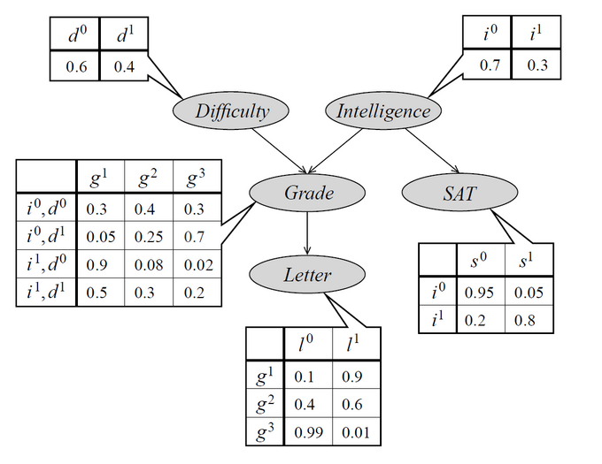
• In many scenarios, it is more practical to use a simple but uncertain rule rather than a complex but certain one, even if the true rule is deterministic and our modeling system has the fidelity to accommodate a complex rule ("most birds fly" versus "birds fly, except for very young birds, sick or injured birds, flightless birds..." etc.).
• There are two kinds of probability:
  • Frequentist: if we repeated an experiment infinitely many times, then proportion $p$ of the repetitions would result in that outcome.
  • Bayesian: the probability represents the degree of belief (i.e. there is a 40% chance that the patient is sick).
• A random variable is a variable that can take on different values randomly. It must be coupled with a probability distribution that specifies how likely each of the states are. Random variables are either discrete or continuous.
• A probability distribution over discrete variables may be described using a probability mass function (PMF). A PMF for a random variable x is denoted $P(x)$. Sometimes we define a variable first, then use $\sim$ notation to specify which distribution it follows later: $x \sim P(x)$.
• PMFs can act on many variables at the same time. Such a function is known as a joint probability distribution. $P(x = \textit{x}, y = \textit{y})$ denotes the probability that $x = \textit{x}$ and $y = \textit{y}$ simultaneously.
• When working with continuous random variables, we use a probability density function (PDF). A PDF does not give the probability of a specific state directly. Instead, the probability of landing inside an infinitesimal region with volume $\delta x$ is given by $p(x)\delta x$. We often denote that $x$ follows the uniform distribution on $[a, b]$ by writing $x\sim U(a, b)$.
• Sometimes we know the probability distribution over a set of variables, and we want to know the probability distribution over just a subset of them. This is known as the marginal probability distribution. For example, if we know $P(x, y)$, we can find $P(x)$ by summing up $P(x = \textit{x}, y = \textit{y})$ for all values of $y$.

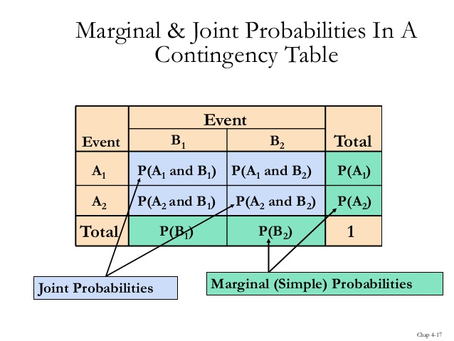
• For continuous variables, we use integration instead of summation.
• In many cases, we are interested in the probability of some event, given that some other event has happened. This is called a conditional probability. We denote the conditional probability that $y =\textit{y}$ given $x = \textit{x}$ as $P(y = \textit{y}\mid x = \textit{x})$.
• Conditional probability explained visually.
• Why do we divide by $P(x = \textit{x})$ in the formula for conditional probability?
• Conditional probability explained with Venn diagrams.
• Any joint probability distribution over many random variables may be decomposed into conditional distributions over only one variable.
• Two random variables $x$ and $y$ are independent if their probability distribution can be expressed as the product of two factors, one involving only $x$ and one involving only $y$. In other words, $p(x = \textit{x}, y = \textit{y}) = p(x = \textit{x})p(y = \textit{y})$.
• Two random variables $x$ and $y$ are conditionally independent given a random variable $z$ if the conditional probability distribution over $x$ and $y$ factorizes in this way for every value of $z$: $p(x = \textit{x}, y = \textit{y}\mid z = \textit{z}) = p(x = \textit{x}\mid z = \textit{z})p(y = \textit{y}\mid z = \textit{z})$.
• Examples of conditional independence.
• The expected value of some function $f(x)$ with respect to a probability distribution $P(x)$ is the average value that $f$ takes on when $x$ is drawn from $P$. Expectations are linear.
• The variance gives a measure of how much the values of a function of a random variable $x$ vary as we sample different values of $x$ from its probability distribution. When the variance is low, the values of $f(x)$ cluster near their expected value. The square root of the variance is known as the standard deviation. The covariance gives some sense of how much two values are linearly related to each other, as well as the scale of these variables. High absolute values of the covariance mean that the values change very much and are both far from their respective means at the same time. If the sign of the covariance is positive, then both variables tend to take on relatively high values simultaneously. If the sign of the covariance is negative, then one variable tends to take on a relatively high value at the times that the other takes on a relatively low value and vice versa.
• Covariance explained visually with overlapping rectangles.
• The covariance matrix is always symmetric. The entries along the diagonal are always variances.
• Note that two variables can be dependent and still have 0 covariance as explained in this post.
• Common probability distributions:
  • Bernoulli: this is a distribution over a single binary random variable. It is controlled by a single parameter $\phi$, which lies in the range $[0, 1]$ and gives the probability of the random variable being equal to 1.
  • Multinoulli: this is a distribution over a single discrete variable with $k$ different states.
  • Gaussian (normal): this applet lets you visualize a normal distribution. Normal distributions are a sensible choice for many applications because many distributions we wish to model are truly close to being normal distributions. Also, the central limit theorem shows that the sum of many independent random variables is approximately normally distributed, as visualized in the following blog post.
  • Multivariate normal distribution: this is a generalization of the normal distribution to $R^{n}$. It involves the Mahalanobis distance in the exponent, which is a way to construct a coordinate system for making measurements by examining the largest axes of variation in the underlying data. See the following forum post for a more detailed explanation.
  • Dirac distribution: this is a distribution that places all of the mass around a single point.
  • Exponential distribution: this is a distribution with a sharp point at $x = 0$. A closely related probability distribution is the Laplace distribution, which allows us to place a sharp peak of probability mass at an arbitrary point.
• The central limit theorem explained on Khan Academy. It states that the sum of many independent random variables is approximately normally distributed.
• Distributions can be combined to form a mixture distribution. On each trial, the choice of which component distribution generates the sample is determined by sampling a component identity from a multinoulli distribution. This model involves a latent variable that we will call $c$ that we cannot observe directly. One powerful type of mixture model is the Gaussian mixture model, in which the components $p(x\mid c = \textit{i})$ are Gaussians. Each component has a separate mean and covariance. A Gaussian mixture model is a universal approximator of densities, in the sense that any smooth density can be approximated with any specific, non-zero amount of error by a Gaussian mixture model with enough components.
• Two useful functions that often arise in a machine learning context are:
  • Sigmoid
  • Softplus
• Bayes' rule states that $P(x\mid y) = P(x)P(y\mid x) / P(y)$. A geometric interpretation of the rule can be found here.
• Information theory is a branch of applied mathematics that revolves around quantifying how much information is present in a signal. The basic idea is that learning that an unlikely event has occurred is more informative than learning that a likely event has occurred (i.e. a message that says "the sun rose this morning" is almost useless, whereas "there was a solar eclipse this morning" is very informative). In general:
  • Likely events should have low information content.
  • Less likely events should have higher information content.
  • Independent events should have additive information.
• The self-information of an event $x = \textit{x}$ is $I(x) = -\log P(x)$. Note that $\log$ is the natural logarithm (base $e$). See the graph of $-\log (x)$ below. Note how events that are more likely having smaller values for $I(x)$:

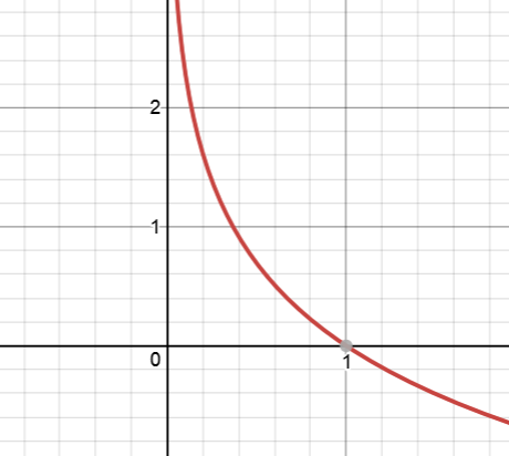
• In the function $I(x)$ above, we refer to the units as nats: one nat is the amount of information gained by observing an event of probability $1/e$.
• The amount of uncertainty in an entire probability distribution is referred to as the Shannon entropy, which is the expected value of $I(x)$. It is usually denoted $H(P)$. It gives a lower bound on the number of bits needed on average to encode symbols drawn from a distribution $P$. Distributions that are nearly deterministic (where the outcome is nearly certain) have low entropy and vice-versa.
• If we have two separate probability distributions $P(x)$ and $Q(x)$ over the same random variable $x$, we can measure how different these two distributions are using the Kullback-Leibler divergence (KL divergence). It is the extra amount of information needed to send a message containing symbols drawn from $P$, when we use a code that was designed to minimize the length of messages drawn from $Q$. In other words, it says how many bits of information we expect to lose by using the distribution $Q$ instead of $P$. KL divergence is explained in great detail in the following article, which discusses how to optimize the parameters of an approximating distribution so that it closely resembles the observed distribution.
• Note that KL divergence is not symmetric, i.e. $D_{KL}(P || Q)\ne D_{KL}(Q || P)$.
• The cross-entropy of two distributions $P$ and $Q$ is $H(P, Q) = -E_{x\sim P}\log Q(x)$. It is similar to KL divergence: minimizing the cross-entropy with respect to $Q$ is equivalent to minimizing the KL divergence because $Q$ does not participate in the omitted term.
• When we represent the factorization of a probability distribution with a graph, we call it a structured probabilistic model or a graphical model. These factorizations can greatly reduce the number of parameters needed to describe a distribution. A detailed tutorial on PGMs can be found here. There are two types of graphical models:
  • Bayesian (directed)
  • Markov (undirected)