Numerical Computation

• Underflow occurs when numbers near zero are rounded to zero. This is problematic because many functions behave differently when their argument is zero rather than a small positive number.
• Overflow occurs when numbers with large magnitude are approximated as positive or negative infinity. Further arithmetic will usually change these infinite values into NaNs.
• As an example, consider the softmax function where all of the $x_{i}$ are equal to some constant $c$. Analytically, we can see that all of the outputs should be equal to roughly $1 / n$. Numerically, this may not occur when $c$ has large magnitude since $\exp(c)$ can underflow or overflow, depending on the sign of $c$. This can be resolved by instead evaluating $softmax(z)$ where $z = x - \max_{i}x_{i}$. Subtracting the largest $x_{i}$ from each element of the vector $x$ results in the largest argument to $\exp$ being 0, which rules out the possibility of overflow. Likewise, at least one term in the denominator will have a value of 1, which rules out the possibility of underflow in the denominator (due to a division by zero).
• Conditioning refers to how rapidly a function changes with respect to small changes in its inputs. The condition number of a matrix is the ratio of the magnitude of its largest and smallest eigenvalues. As a simple example, imagine that we are trying to solve the linear system of equations $Ax = b$. Now, imagine $A$ is a scalar. If $A$is very small, then its inverse is very large. Then, even a small error in the data $b$ gets amplified by the large inverse of $A$ in the equation $x = A^{-1}b$. For a walk-through example of ill-conditioned matrices, see the following article.
• Most deep learning algorithms involve optimization of some sort. The function we want to minimize or maximize is called the objective function or criterion. When we are minimizing it, we may also call it the cost function, loss function, or error function. We often denote the value that minimizes or maximizes a function with a superscript $*$. For example, $x^{*} = \arg\min f(x)$.
• Points where the derivative of a function is 0 provide no information about which direction to move during gradient descent. These are known as critical points or stationary points. A local minimum is a point where $f(x)$ is lower than all neighboring points, so it is no longer possible to decrease $f(x)$ by making infinitesimal steps.
• A point that obtains the absolute lowest value of $f(x)$ is a global minimum. In deep learning, we usually settle for finding a value of $f$ that is very low but not necessarily minimal in any formal sense.
• The gradient is a multi-variable generalization of the derivative. It is a vector-valued function that operates on functions of several variables. We can decrease a function $f$ by moving in the direction of the negative gradient. The directional derivative tells us how the value of the function $f$ changes if we take a small step in some direction $u$. Note that if the directional derivative is used to compute slope, $u$ must be a unit vector. It is outlined in detail in the following Khan Academy article.
• Sometimes we need to find all of the partial derivatives of a function whose input and output are both vectors. The matrix containing all such partial derivatives is known as the Jacobian matrix.
• The second derivative of a function is a measure of curvature:When our function has multiple input dimensions, there are many second derivatives. These derivatives can be collected together into a matrix called the Hessian matrix. The Hessian is the Jacobian of the gradient. It is explained in detail in the following Khan Academy video.
  • In the case of negative curvature, the cost function actually decreases faster than the gradient predicts.
  • In the case of no curvature, the gradient predicts the decrease correctly.
  • In the case of positive curvature, the cost function decreases slower than expected and eventually begins to increase, so too large of step sizes can actually increase the function inadvertently.
• Anywhere that the second partial derivatives are continuous, the differential operators are commutative (their order can be swapped by Schwarz's theorem). The Hessian matrix is symmetric at such points. Most of the functions we encounter in the context of deep learning have a symmetric Hessian almost everywhere.
• What is the difference between the gradient, Jacobian, and Hessian?
• In multiple dimensions, we can determine whether a critical point is a local minimum, local maximum, or a saddle point by examining the eigenvalues of the Hessian matrix:
  • The observations above stem from the fact that the Hessian matrix is symmetric and therefore has an orthogonal basis of eigenvectors. If all of the eigenvalues of the Hessian are positive, for example, then we can show through the basic properties of matrix-vector multiplication that the product $Hv$ for any vector $v$ will be positive (to see this, write $v$ as a linear combination of the eigenvectors of $H$). This implies that the function has positive curvature everywhere around the point in question.
  • If the Hessian is positive definite, the point is a local minimum.
  • The second derivative test is inconclusive when all of the non-zero eigenvalues have the same sign but at least one eigenvalue is zero.
  • If the Hessian is negative definite, the point is a local maximum.
  • When at least one eigenvalue is positive and at least one eigenvalue is negative, we know that the point is a local maximum on one cross section but a local minimum on another cross section.
• The condition number of the Hessian measures how much the second derivatives vary. When the Hessian has a poor condition number, gradient descent performs poorly because the derivative increases rapidly in one direction and slowly in another.
• Newton's method is an iterative algorithm for finding the points where a function equals zero. To keep things simple, let's consider a scalar function $f(x)$. We want to find the point(s) where $f(x) = 0$. So, we start with some initial value of $x$, and at each time step $t$, we calculate: $x^{t + 1} = x^{t} - f(x^{t}) / f'(x^{t})$. This is equivalent to finding the point where the tangent line at $x^{t}$ equals 0. Remember, $y = mx + b$, so if $0 = mx + b$, then $x$ must equal $-b / m$.
• When applied to optimization, it lets us find the minima or maxima of a function. It is a second-order method, as opposed to gradient descent, which is a first-order method. To do this, we follow the same procedure outlined above except we use a second-order approximation of the function at each point $x^{t}$. At each time step $t$, we calculate $x^{t + 1} = x^{t} - f'(x^{t}) / f''(x^{t})$. This amounts to finding the minimum of a quadratic (parabola) at each $x^{t}$. This process can be extended to multivariable functions, as outlined in the following video.
• How do you derive the second-order Taylor series expansion for a multivariable function?
• In the context of deep learning, we sometimes gain some guarantees by restricting ourselves to functions that are Lipschitz continuous, meaning functions whose rate of change is bounded by a Lipschitz constant. This is useful because it allows us to quantify our assumption that a small change in the input made by an algorithm such as gradient descent will have a small change in the output.
• Sometimes we wish to find the maximal or minimal value of $f(x)$ for values of $x$ in some particular set $S$. This is known as constrained optimization. We often wish to find a solution that is small in some sense. A common approach in such situations is to impose a norm constraint (i.e. the length of each vector $x$ is less than or equal to 1). A visual explanation of a simple constrained optimization problem can be found in the following Khan Academy video. It also explains why the local maximum corresponds to the value where the contour lines of the function lie tangent to the constraint region. The basic idea is, at the point where the contour lines of the constraint region are tangent to the contour lines of the function $f$, the gradients of the two functions are related by some constant known as the Lagrange multiplier. In other words, the gradients will be pointing in the same direction but might have different lengths.
• Lagrange multipliers explained.
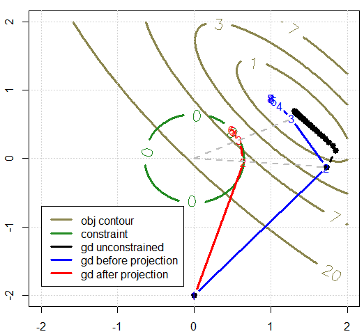
• One simple approach to constrained optimization is to modify gradient descent, taking the constraint into account. We can make gradient descent steps then project the result back into $S$. This is depicted graphically below (explained in the following forum post):

• What is the difference between projected gradient descent and gradient descent?
• The Karush-Kuhn-Tucker (KKT) approach provides a very general solution to constrained optimization. With this approach, we introduce a new function called the generalized Lagrangian function (this concept is also introduced in the Khan Academy articles linked above). To define the Lagrangian, we first need to describe S in terms of equalities and inequalities. The KKT approach is explained in the following article.
• Aside: what is the difference between the "arg min" notation and "min"?
  • $\arg\min$: produces the input value (like $x$) where the minimum is obtained
  • $\min$: produces the minimum value of the function