Regularization for Deep Learning

• In the context of deep learning, most regularization strategies are based on regularizing estimators, which works by trading increased bias for reduced variance.

An effective regularizer is one that makes a profitable trade, reducing variance significantly while not overly increasing the bias.

• In practice, an overly complex model family does not necessarily include the target function or the true data-generating process, or even a close approximation of either. The data-generating process is the true, underlying phenomenon that is creating the data. The model is the (often imperfect) attempt to describe and emulate the phenomenon, as described in the following Quora post.
• Many regularization approaches are based on limiting the capacity of models by adding a parameter norm penalty $\Omega (\theta)$ to the objective function $J$. We denote the regularized objective function by $\widetilde{J}$:

$\widetilde{J}(\theta ; X, y) = J(\theta ; X, y) + \alpha \Omega (\theta)$

• Generally, we choose a parameter norm penalty that penalizes _only the weights _of the network and leaves the biases unregularized. This is because the bias parameters don't contribute to the curvature of the model, so there is no point in regularizing them. The learning algorithm cannot put arbitrarily large values for the bias term since this will result in a grossly large loss value. In other words, given some training set, the learning algorithm cannot move the separating hyperplane arbitrarily far away from the true one.
• The $L^{2}$ parameter norm penalty is commonly known as weight decay. This regularization strategy drives the weights closer to the origin by adding a regularization term $\Omega (\theta) = \frac{1}{2}||w||_{2}^{2}$ to the object function. It is sometimes referred to as ridge regression.
• When using weight decay, a single gradient step to update the weights involves multiplicatively shrinking the weight vector by a constant factor. If we let $w^{*}$denote the value of the weights that obtains minimal unregularized training cost, then we can show that the effect of weight decay is to rescale $w^{*}$along the axes defined by the eigenvectors of the Hessian matrix $H$.

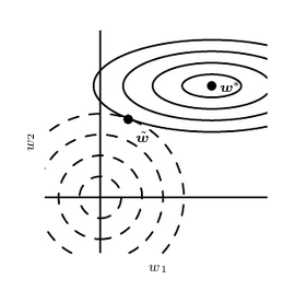
• Only directions along which the parameters contribute significantly to reducing the objective function ($w_{2}$ in the image above) are preserved relatively intact. In directions that do not contribute to reducing the objective function ($w_{1}$ in the image above), a small eigenvalue of the Hessian tells us that movement in this direction will not significantly increase the gradient. Components o the weight vector corresponding to such unimportant directions are decayed away through the use of the regularization throughout training.
• We can also study the effect of $L^{2}$ regularization on a simple model like linear regression.
  • The cost function with regularization can be written as $(Xw - y)^{T}(Xw - y) + \frac{1}{2}\alpha w^{T}w$, where $X$ is the training data.
  • This changes the normal equations for the solution from $w = (X^{T}X)^{-1}X^{T}y$ to $w = (X^{T}X + \alpha I)^{-1}X^{T}y$.
  • The matrix $X^{T}X$ is proportional to the covariance matrix $\frac{1}{m}X^{T}X$. This follows from the fact that if the vectors (i.e. rows of $X$) are centered random variables, then the Gram matrix (which is $X^{T}X$) is approximately proportional to the covariance matrix, with the scaling determined by the number of elements in the vector (which is $m$).
  • The new matrix in the parenthesis is the same as the original one but with the addition of $\alpha$ to the diagonal. The diagonal entries of this matrix correspond to the variance of each input feature. We can see that $L^{2}$ regularization causes the learning algorithm to "perceive" the input $X$ as having higher variance, which makes it shrink the weights on features whose covariance with the output target is low compared to this added variance.
• In comparison to $L^{2}$ regularization, $L^{1}$ regularization results in a solution that is more sparse for a large enough $\alpha$. Sparsity in this context refers to the fact that some parameters have an optimal value of zero. An explanation of why $L^{1}$ regularization is sparsity inducing can be found in the following post.
  • This sparsity inducing property is used extensively as a feature selection mechanism.

$L^{1}$ regularization will move any weight towards 0 with the same step size, regardless of the weight's value. In contrast, $L^{2}$ regularization will also move any weight towards 0, but it will take smaller and smaller steps as the weight's value approaches 0.

• In this section, the author makes use of a quadratic approximation to the objective function. This is a second-order Taylor series approximation, in the multivariable case. Using a Taylor series, we can approximate a function around the neighborhood of some point $a$ (in the scalar case). If we are dealing with some multivariable function $f(x, y)$, we could form a second-order approximation of $f$ around some point $(a, b)$ as follows:

$f(x, y) = f(a, b) + f_{x}(a, b)(x - a) + f_{y}(a, b)(y - b) + \frac{1}{2}[f_{xx}(a, b)(x - a)^{2} + 2f_{xy}(a, b)(x - a)(y - b) + f_{yy}(y - b)^{2}]$

• If we now let $x = \langle x, y\rangle$ and $a = \langle a, b\rangle$, this can be written more compactly as:

$f(x) = f(a) + [(x - a)$$f(x) = f(a) + [(x - a)\cdot \bigtriangledown f(a)] + \frac{1}{2}[(x - a)\cdot (H(x)\cdot (x - a))]$

• A full, worked-out example of a second-order Taylor series approximation for a function of two variables can be found here.
• Many regularization strategies can be interpreted as MAP Bayesian inference. This is covered in detail in the following post.
  • $L^{2}$ regularization is equivalent to MAP with a Gaussian prior on the weights.
  • $L^{1}$ regularization is equivalent to MAP with an isotropic Laplace distribution as a prior (after ignoring some terms that do not depend on the weights $w$).
  • Regularization is the process of introducing additional information in order to solve ill-posed problems or prevent overfitting. A trivial example is trying to fit a simple linear model to a dataset that only contains a single point. In this case, you can't estimate both the slope and the intercept (you need at least two points), so any MLE estimate (which only uses the data) will be ill-formed. Instead, if you provide some "additional information" (i.e. prior information), you can get a much more reasonable estimate.
  • Again, in Bayesian inference, we're primarily concerned with the posterior: "the probability of the parameters given the data."
  • The prior is something that we explicitly choose that is not based on the data. Even in cases where we don't know anything about the nature of the true data-generating process, we can choose a weak prior, which will only bias the result slightly from the MLE estimate.
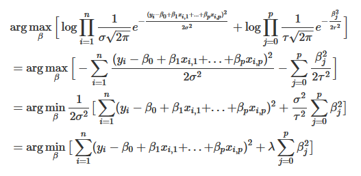
  • We can see the effect of introducing a normally distributed prior on each of the parameters $\beta_{i}$ in a linear regression model below.

• A list of various regularization strategies can be found in the following Wikipedia article.
• We can view the normal penalties described above as a form of constrained optimization.
  • If we are using $L^{2}$ regularization, then the weights are constrained to lie in an $L^{2}$ ball.
  • If we are using $L^{1}$ regularization, then the weights are constrained to lie in a region of limited $L^{1}$ norm.
  • The hyperparameter $\alpha$ controls the size of the constraint region.
• We can also use explicit constraints rather than penalties. An example of this is projected gradient descent. Penalties such as the weight decay strategies discussed above can cause non-convex optimization procedures to get stuck in local minima corresponding to small $\theta$.
• Regularization can also be used to solve underdetermined problems. An example of this is logistic regression applied to a problem where the classes are linearly separable. If a weight vector $w$ is able to achieve perfect classification, then $2w$ will also achieve perfect classification and higher likelihood.
  • Usually, high-dimensional problems are underdetermined because the sample size is much smaller than the number of features. Therefore, some constraints are necessary in order to make the problem determined.
  • Regularization makes the intrinsic dimensionality of the problem small so that it remains solvable in the high-dimensional space.
  • This process is explained in the following post.
• The best way to make a machine learning model generalize better is to train it on more data. One way to do this is through data augmentation, which typically involves applying some transformations to the input $x$.
  • Injecting noise into the input of a neural network can also be seen as a form of data augmentation.
  • Noise injection also works when the noise is applied to the hidden units, which can be seen as doing data augmentation at multiple levels of abstraction.
  • Dropout can be viewed as a process of constructing new inputs by multiplying by noise.
• Another way that noise has been used in the service of regularizing models is by adding it to the network weights, which encourages stability. This form of regularization encourages the parameters to go to regions of parameter space where small perturbations of the weights have a relatively small influence on the output. In other words, it pushes the model into regions where the model is relatively insensitive to small variations in the weights. The following blog post explains why randomness is important in deep learning.
• Noise can also be applied to the output targets. Label smoothing regularizes a model based on a softmax with $k$ output values by replacing the hard 0 and 1 classification targets with targets of $\frac{\epsilon}{k - 1}$ and $1 - \epsilon$, respectively. The standard cross-entropy loss may then be used with these soft targets.
• Semi-supervised learning refers to learning a representation $h = f(x)$. The goal is to learn a representation so that examples from the same class have similar representations. A linear classifier in the new space may achieve better generalization in many cases.
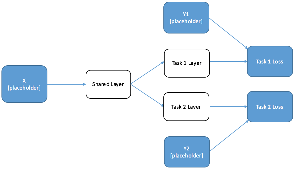
• Multitask learning is a way to improve generalization by pooling the examples arising out of several tasks. From the point of view of deep learning, the underlying prior belief is the following: among the factors that explain the variations observed in the data associated with different tasks, some are shared across two or more tasks.

• When training large models with sufficient representational capacity to overfit a task, we often observe that the training error decreases steadily over time, but the validation error begins to rise again. To combat this, we can use a technique known as early stopping.
  • Every time the error on the validation set improves, we store a copy of the model parameters. When the training algorithm terminates, we return these parameters rather than the latest parameters.
  • The algorithm terminates when no parameters have improved upon the best recorded validation error for some pre-specified number of iterations.
  • Early stopping can be used alone or in conjunction with other regularization strategies.
  • Under certain conditions, it can be shown that early stopping and $L^{2}$ regularization are equivalent.
  • In $L^{2}$ regularization, parameter values corresponding to directions of significant curvature (of the objective function) are regularized less than directions of less curvature. In the context of early stopping, this means that parameters that correspond to directions of significant curvature tend to learn early relative to parameters corresponding to directions of less curvature.

Early stopping has the advantage over weight decay in that it automatically determines the correct amount of regularization while weight decay requires many training experiments with different values of its hyperparameter.

• The regularization strategies discussed thus far work by adding constraints or penalties to the model parameters with respect to a fixed region or point. For example, $L^{2}$ regularization penalizes the model parameters for deviating from the fixed value of zero. Instead, we might want to ensure that certain parameters are close to one another. This is known as parameter sharing.
  • The most popular and extensive use of parameter sharing occurs in CNNs. This technique allows CNNs to be translation invariant.
  • Parameter sharing can also dramatically lower the number of unique model parameters.
• Weight decay acts by placing a penalty directly on the model parameters. Another strategy is to place a penalty on the activations of the hidden units, encouraging them to be sparse.
  • Note that this is not the same as $L^{1}$ regularization, which induces a sparse parametrization (meaning that many of the weights become zero or close to zero).
  • The difference is illustrated in the image below, where $7.46$ is an illustration of a sparsely parametrized linear regression model and $7.47$ is a linear regression model with a sparse representation $h$ of the data $x$.
  • Representational regularization is achieved by the same sorts of mechanisms that we have used for parameter regularization.
  • Other approaches obtain representational sparsity by placing a hard constraint on the activation values. Orthogonal matching pursuit (OMP-k) encodes an input $x$ with the representation $h$ that solves a constrained optimization problem, which is explained in the following tutorial. Essentially, the algorithm tries to find a representation wtih less than $k$ non-zero entries.

• Bagging (bootstrap aggregating) is a technique for reducing generalization error by instantiating and training several different models. At test time, all of the models vote on the output. This is an example of an ensemble method.
  • It can be shown that, on average, an ensemble will perform at least as well as any of its members, and if the members make independent errors, the ensemble will perform significantly better than its members.
  • Bagging involves constructing $k$ different datasets. Each dataset has the same number of examples as the original dataset, but each dataset is constructed by sampling with replacement from the original dataset. This means that, with high probability, each dataset will be missing some of the examples from the original dataset and will contain several duplicated examples.

Any machine learning algorithm can benefit substantially from model averaging at the price of increased computation and memory.

• Dropout can be thought of as a method of making bagging practical for ensembles of very many large neural networks. Specifically, dropout trains the ensemble consisting of all sub-networks that can be formed by removing non-output units from an underlying base network.
  • Each time we load a minibatch, we randomly sample a different binary mask to apply to all of the input and hidden units in the network. The mask for each unit is sampled independently from all of the others.
  • To make a prediction, a bagged ensemble must accumulate votes from all of its members. Each model $i$ produces a probability distribution $p^{(i)}(y\mid x)$. The prediction of the ensemble is given by the arithmetic mean of all of these distributions.
  • In the case of dropout, each sub-model defined by a mask vector $\mu$ defines a probability distribution $p(y\mid x, \mu)$. Because the arithmetic mean over all masks includes an exponential number of terms, it is intractable to evaluate except when the structure of the model permits some form of simplification.
  • Instead, we can approximate the inference with sampling (10 to 20 different masks) by averaging together the output from many masks.
  • An even better approach requires only a single forward pass. To do so, we use the geometric mean rather than the arithmetic mean of the ensemble members' predicted distributions.
    • The geometric mean is defined as the $n$-th root of the product of $n$ numbers.
    • A geometric mean is often used when comparing items with vastly different scales. For example, it can be used to give a meaningful "average" to compare two companies which are rated from 0 to 5 for their environmental sustainability and 0 to 100 for their financial viability. If an arithmetic mean were used, the "financial viability" term would be given more weight simply because its numeric range is larger.
  • A key insight is that we can approximate the ensemble with a single model: the model with all units but with the weights going out of unit $i$ multiplied by the probability of including unit $i$.
  • Dropout has several advantages.
    • It is very computationally cheap.
    • It does not significantly limit the type of model or training procedure that can be used. Many other regularization strategies of comparable power impose more severe restrictions on the architecture of the model.
  • One of the other key insights of dropout is that training a network with stochastic behavior and making predictions by averaging over multiple stochastic decisions implements a form of bagging with parameter sharing. We can think of any form of modification parametrized by a vector $\mu$ as training an ensemble consisting of $p(y\mid x, \mu)$ for all possible values of $\mu$. In fact, it has been shown that multiplying the weights by values drawn from a normal distribution can outperform dropout based on binary masks (see section 10 of the follow paper).

A large portion of the power of dropout arises from the fact that the masking noise is applied to the hidden units. This can be seen as a form of highly intelligent, adaptive destruction of the information content of the input rather than destruction of the raw values of the input. For example, if the model learns a hidden unit that detects a face by finding a nose, then dropping that unit corresponds to erasing the information that there is a nose in the image. The model must learn another hidden unit that either redundantly encodes the presence of a nose or detects the face by another feature, such as the mouth.

• Adversarial training discourages highly sensitive, locally linear behavior by encouraging the network to be locally constant in the neighborhood around the training data. This can be seen as a way of explicitly introducing a local constancy prior into supervised neural networks. The assumption is that different classes usually lie on disconnected manifolds, and a small perturbation should not be able to jump from one class manifold to another class manifold.
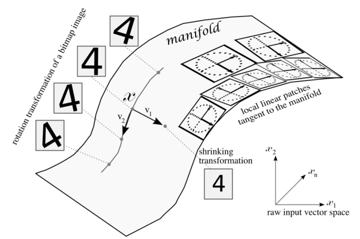
• Many machine learning algorithms aim to overcome the curse of dimensionality by assuming that the data lies near a low-dimensional manifold (as described in chapter 5). The tangent prop algorithm trains a classifier with an extra penalty to make each output of the neural network locally invariant to known factors of variation. These factors of variation correspond to movement along the manifold near which examples of the same class concentrate. Local invariance is achieved by requiring the gradient of the network's output with respect to its input to be orthogonal to the known manifold tangent vectors $v^{(i)}$ at $x$.
  • Tangent propagation is closely related to dataset augmentation, which is covered in the following blog post. In both cases, the user of the algorithm encodes his or her prior knowledge of the task by specifying a set of transformations that should not alter the output of the network.
  • The difference is that in the case of dataset augmentation, the network is explicitly trained to correctly classify distinct inputs that were created by applying more than an infinitesimal amount of these transformations.
  • Tangent propagation does not require explicitly visiting a new input point. Instead, it analytically regularizes the model to resist perturbation in the directions corresponding to the specified transformation.
• Tangent propagation and dataset augmentation using manually specified transformations both require that the model be invariant to certain specified directions of change in the input. Double backprop and adversarial training both require that the model should be invariant to _all _directions of change in the input as long as the change is small.

Just as dataset augmentation is the non-infinitesimal version of tangent propagation, adversarial training is the non-infinitesimal version of double backprop.

• The manifold tangent classifier eliminates the need to know the tangent vectors a priori. These estimated tangent vectors go beyond the classical invariants that arise out of the geometry of images (such as translations, rotations, and scaling) and include factors that must be learned because they are object-specific (such as moving body parts).
  • Autoencoders can estimate the manifold tangent vectors.